Why Should I Lock Cells in Google Sheets?
By locking a cell, you can restrict its editing permissions. When a cell is locked, no one else can edit it except you and the people you authorize to do so. This functionality is extremely useful, especially when collaborating with others or working as a team. Below are some example case scenarios wherein locking a cell would be the best thing to do:
You’re working on a group project wherein you need to make sure that the entries you’ve made remain unchanged or unaltered. You are doing a work collaboration for one particular worksheet. To prevent accidental editing or deletion, you decided to lock the cells containing extremely valuable information. You need to update the formatting of an entire column in which there are specific cells that should be left unchanged.
How Do I Lock a Cell in Google Sheets?
Locking cells in Google Sheets is easy. All you need to do is learn to lock cells using the “Protect range” option. To do this, you can choose from any of the methods listed below:
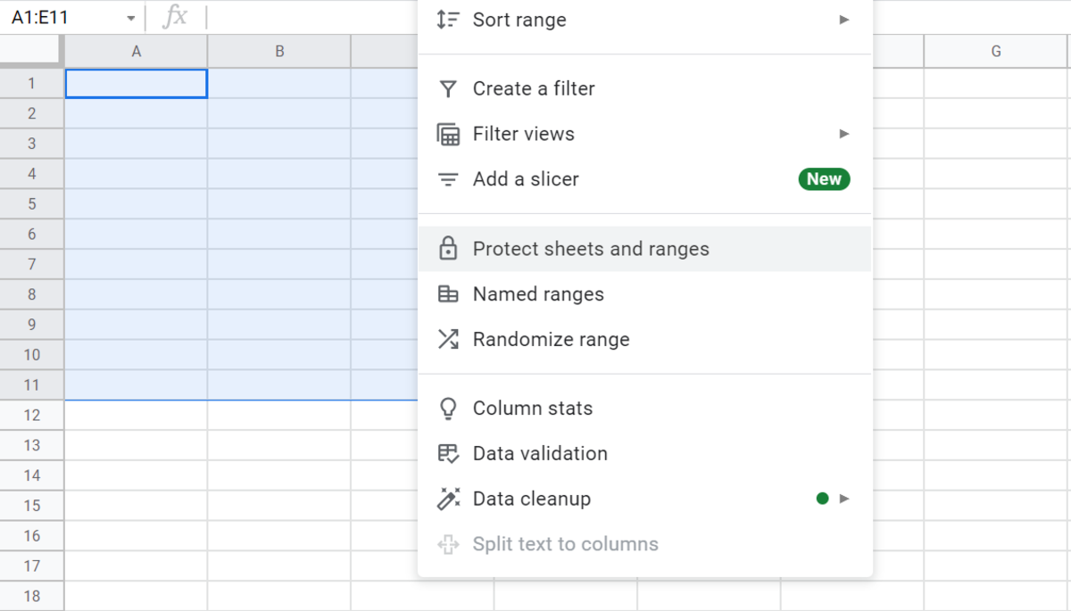
Method 1: Right-Click Option
This option works best when you want to lock multiple cells so you don’t have to manually enter the cell range. What you need to do is: That’s it!
Method 2: Data Tab Option
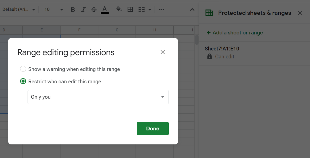
The second option is ideal for locking cells that you cannot easily highlight or select using your mouse. To lock cells from the Data tab, you simply need to do the following: Once you’ve locked the cells, no one else can edit or alter these cells except you and the users you’ve allowed to have editing permissions.
How Do I Unlock Cells in Google Sheets?
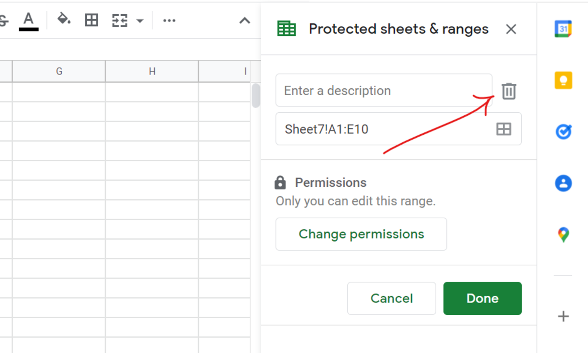
Unlocking cells in Google Sheets is simply doing the opposite of the steps above. The easiest way to do this is to follow the second method. Instead of setting permissions, you find the cells or range of cells you want to unlock and then click the delete icon. Once deleted from the protected sheets and ranges list, the cell will immediately revert to its default permissions.
How Do I Lock Columns and Rows in Google Sheets?
If locking a cell in Sheets won’t suffice. You can lock the entire row or column instead. Locking an entire row or column is easier since you don’t need to enter or define a cell range. Select the rows or columns that you want to lock and then go to View > Freeze. Make your selection based on how many cells or rows you want to freeze. That’s it! Note that freezing a row or column won’t make it uneditable. It will just “freeze” the column or row so, when you scroll the sheet, the column or row will remain in its fixed position.
How Do I Lock an Entire Sheet in Google Sheets?
If locking rows and columns still won’t suffice, you can always choose to lock an entire sheet. To lock an entire sheet, click the arrow next to the sheet title and then click “Protect Sheet.” Enter a description and then click “Set permissions.” Adjust the permission settings according to whom you want to view and edit the sheet. Click “Done.” Once a sheet is locked, you can always change or update its permissions whenever you want.
Protect Your Worksheet by Knowing How to Lock and Unlock Cells
Knowing how to lock and unlock a cell in Google Sheets allows you to protect the changes you’ve made to your worksheet. Oftentimes, in group projects, there are instances wherein the data or sheet formatting has been altered by accident. Yes, you may be able to restore the sheet by reverting to a previous version, but that involves a tedious process of going into the sheet’s version history. A much more straightforward approach would be to lock the cells so that nobody else can edit them unless they have permission. This content is accurate and true to the best of the author’s knowledge and is not meant to substitute for formal and individualized advice from a qualified professional. © 2022 Kent Peligrino